4.4 Capturing trend changes in the past

ASMODEE implicitly assumes that the fitting set can be used to capture a single trend. It frequently happens, however, that this time period actually saw a change in trend, which then cannot be captured by a simple model (e.g. Figure 4.3).

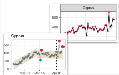
Example of trend change in COVID-19 data. This figure illustrates a case of change in temporal trends having occured during the *fitted* time period in the raw data (red dots and plain black line) captured by ASMODEE (grey dots and model envelope).

Figure 4.3: Example of trend change in COVID-19 data. This figure illustrates a case of change in temporal trends having occured during the fitted time period in the raw data (red dots and plain black line) captured by ASMODEE (grey dots and model envelope).

The strategy we employ to address this issue is to:

define a breaking point date marking the change in trend
building a categorical variable period marking dates before and after
using an interaction term for the effect of time (variable date) combined with period so that the model will fit a slope before and after the changing point

In practice, we often ignore how to define 1). This can be addressed by generating many models, each with a different breaking point, and leaving to ASMODEE the task to select the best fitting model.

This approach is not entirely straightforward to implement; we illustrate it below:


# generate some dates for the example
some_dates <- as.Date("2021-02-04") + 0:30
some_dates
##  [1] "2021-02-04" "2021-02-05" "2021-02-06" "2021-02-07" "2021-02-08"
##  [6] "2021-02-09" "2021-02-10" "2021-02-11" "2021-02-12" "2021-02-13"
## [11] "2021-02-14" "2021-02-15" "2021-02-16" "2021-02-17" "2021-02-18"
## [16] "2021-02-19" "2021-02-20" "2021-02-21" "2021-02-22" "2021-02-23"
## [21] "2021-02-24" "2021-02-25" "2021-02-26" "2021-02-27" "2021-02-28"
## [26] "2021-03-01" "2021-03-02" "2021-03-03" "2021-03-04" "2021-03-05"
## [31] "2021-03-06"

# build a dummy dataset
library(magrittr)
library(dplyr)

x <- tibble(date = some_dates) %>%
  mutate(day = as.integer(date - min(date)))

# build all changepoint variables between 10 and 20 days
min_k <- 5
max_k <- 25
k_values <- min_k:max_k
df_changepoints <- lapply(k_values,
                       function(k)
                         x %>%
                         transmute(if_else(day <= k, "before", "after")) %>%
                         pull(1)) %>%
  data.frame() %>%
  tibble() %>%
  setNames(paste0("change_", k_values))

# add changepoint variables to main data
x <- x %>%
  bind_cols(df_changepoints)
x
## # A tibble: 31 x 23
##    date         day change_5 change_6 change_7 change_8 change_9 change_10
##    <date>     <int> <chr>    <chr>    <chr>    <chr>    <chr>    <chr>    
##  1 2021-02-04     0 before   before   before   before   before   before   
##  2 2021-02-05     1 before   before   before   before   before   before   
##  3 2021-02-06     2 before   before   before   before   before   before   
##  4 2021-02-07     3 before   before   before   before   before   before   
##  5 2021-02-08     4 before   before   before   before   before   before   
##  6 2021-02-09     5 before   before   before   before   before   before   
##  7 2021-02-10     6 after    before   before   before   before   before   
##  8 2021-02-11     7 after    after    before   before   before   before   
##  9 2021-02-12     8 after    after    after    before   before   before   
## 10 2021-02-13     9 after    after    after    after    before   before   
## # … with 21 more rows, and 15 more variables: change_11 <chr>, change_12 <chr>,
## #   change_13 <chr>, change_14 <chr>, change_15 <chr>, change_16 <chr>,
## #   change_17 <chr>, change_18 <chr>, change_19 <chr>, change_20 <chr>,
## #   change_21 <chr>, change_22 <chr>, change_23 <chr>, change_24 <chr>,
## #   change_25 <chr>

Once these variables have been created, one can build the corresponding models using the same approach as before:


library(trending)

# step 1
mod_content <- paste("date * change", k_values, sep = "_")
mod_content
##  [1] "date * change_5"  "date * change_6"  "date * change_7"  "date * change_8" 
##  [5] "date * change_9"  "date * change_10" "date * change_11" "date * change_12"
##  [9] "date * change_13" "date * change_14" "date * change_15" "date * change_16"
## [13] "date * change_17" "date * change_18" "date * change_19" "date * change_20"
## [17] "date * change_21" "date * change_22" "date * change_23" "date * change_24"
## [21] "date * change_25"

# step 2
models_txt <- sprintf("glm_model(cases ~ %s, family = poisson)", mod_content)

# step 3
models <- lapply(models_txt, function(e) eval(parse(text = e)))
class(models) # this is a list
## [1] "list"
length(models) # each component is a model
## [1] 21
models %>%
  head(4) %>% # only check for 4 models
  lapply(get_formula) # check formulas
## [[1]]
## cases ~ date * change_5
## <environment: 0x562476667b28>
## 
## [[2]]
## cases ~ date * change_6
## <environment: 0x56247667b048>
## 
## [[3]]
## cases ~ date * change_7
## <environment: 0x562476756518>
## 
## [[4]]
## cases ~ date * change_8
## <environment: 0x562476765830>

Note that of course, changes in trend may happen in conjunction with other processes, such as periodicity (e.g. Figure 4.4). In such cases, the approach illustrated at the beginning of this chapter can be used to generate model contents with/without change and with/without periodic effect.

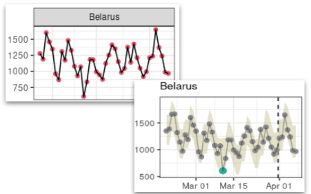
Example of trend change with periodicity in COVID-19 data. This figure illustrates a case of change in temporal trends having occured during the *fitted* time period, combined with weekly periodicity in the raw data (red dots and plain black line) captured by ASMODEE (grey dots and model envelope).

Figure 4.4: Example of trend change with periodicity in COVID-19 data. This figure illustrates a case of change in temporal trends having occured during the fitted time period, combined with weekly periodicity in the raw data (red dots and plain black line) captured by ASMODEE (grey dots and model envelope).